Joint modelling of longitudinal and survival data

This post gives a gentle introduction to the joint longitudinal-survival model framework, and covers how to fit such models using our merlin command in Stata.

A joint model consists of a continuous, repeatedly measured (longitudinal) outcome, and a time-to-event outcome, with their two submodels linked by random effects, or functions of them. Let’s formally define everything we need.

For the ith patient, we have the observed longitudinal outcome measured at time t, $y_{i} (t)$ ,

y_{i} (t) = m_{i} (t) + ϵ_{i} (t)

where

m_{i} (t) = X_{1 i} (t) β_{1} + Z_{i} (t) b_{i}

and $ϵ_{i} (t)$ is our normally distributed residual variability (measurement error). We call $m_{i} (t)$ our trajectory function, representing the true underlying value of the continuous outcome at time t, which is a function of fixed and random effects with associated design matrices, $X_{1 i} (t)$ and $Z_{i} (t)$ , and coefficients and random effects, $β_{1}$ and $b_{i}$ , respectively. We assume normally distributed random effects,

b_{i} ~ N (0, Σ) .

Our survival model can be defined in terms of the hazard function,

h_{i} (t) = h_{0} (t) \exp (X_{2 i} β_{2} + α m_{i} (t))

where $h_{0} (t)$ is the baseline hazard function, and $X_{2 i}$ is a vector of baseline covariates with associated log hazard ratios $β_{2}$ . We can then link the current value of the biomarker directly to survival, where $α$ is a log hazard ratio for a one-unit increase in the biomarker, at time t. This is just one way of linking the models…keep reading.

Let’s assume a random intercept and random linear trend for the biomarker trajectory and a further fixed effect of time squared to allow for more flexibility, i.e.

m_{i} (t) = (β_{10} + b_{0 i}) + (β_{11} + b_{1 i}) t + β_{12} t^{2}

Our longitudinal model can be as simple or complex as we need, both in terms of fixed and random effects.

Simulating the data

Rather than analyse a real dataset, we’ll simulate one from exactly this joint model, so we know what merlin should find. We start by setting a seed (as we always should), generating 400 patients, and randomising each of them to treatment (trt) with probability 0.5.

Stata

. clear

. set seed 2461

. set obs 400
Number of observations (_N) was 0, now 400.

. gen id = _n

. gen trt = runiform() > 0.5

Next, we generate each patient’s random intercept and random slope, $b_{0 i}$ and $b_{1 i}$ , drawing them from a bivariate normal distribution with standard deviations 1 and 0.2 and a correlation of 0.4, using drawnorm.

Stata

. matrix Sigma = (1, 0.08 \ 0.08, 0.04)     // SDs 1 and 0.2, correlation 0.4

. drawnorm b0 b1, cov(Sigma)

Now the survival times, which we simulate from the current value model above. The baseline hazard is Weibull, $h_{0} (t) = λ γ t^{γ - 1}$ , with $λ = 0.02$ and $γ = 1.2$ , treatment has a log hazard ratio of $β_{2} = - 0.5$ , and the association with the current value of the trajectory is $α = 0.8$ , where

m_{i} (t) = (0.5 + b_{0 i}) + (0.1 + b_{1 i}) t + 0.01 t^{2}

Because the hazard depends on a trajectory that changes over time, there’s no closed-form cumulative hazard to invert, but avalon, the merlin family’s simulator, does the numerical integration and root-finding for us (Crowther and Lambert, 2013). We give avalon user the hazard as a function of time, {t}, written with Mata’s element-wise colon operators, and the treatment effect in its covariates() option. Anyone still alive at 10 years is censored there.

Stata

. avalon user stime died,                           /// new variables
>         hazard(0.02:*1.2:*{t}:^(1.2-1)            /// Weibull baseline
>                :* exp(0.8 :*                      /// alpha x current value
>                (0.5 :+ b0 :+ (0.1 :+ b1):*{t}     ///   trajectory m_i(t)
>                 :+ 0.01:*{t}:^2)))                ///
>         covariates(trt -0.5)                      /// treatment effect
>         maxtime(10)                               //  admin. censoring
note: this hazard is close to singular at the lower limit.
      Gauss-Kronrod puts the 15-point quadrature error at  1.4e-02; the run
      used nodes() points and is better than that, but in the same regime. Raisi
> ng
      nodes() helps only slowly here -- see r(qerror).

avalon adds a note that the hazard is close to singular at the lower limit, and that more quadrature nodes help only slowly. It is a cautious check, and here a harmless one: rerunning with nodes(200) instead of the default gives the same simulated times, to within 1e-12.

The biomarker is measured at entry and then annually, until death or censoring, with normally distributed measurement error with a standard deviation of 0.35. The easiest way to do that is to expand the data to ten rows per patient, and drop the visits that fall after each patient’s event or censoring time.

Stata

. expand 10
(3,600 observations created)

. bys id : gen time = _n - 1

. drop if time > stime
(928 observations deleted)

. gen y = 0.5 + b0 + (0.1 + b1)*time + 0.01*time^2 + rnormal(0, 0.35)

merlin works with each outcome’s data side by side: the biomarker has a row per measurement, but the survival outcome needs only one row per patient, so we blank out its repeats.

Stata

. bys id (time) : replace stime = . if _n > 1
(2672 real changes made, 2672 to missing)

. bys id (time) : replace died = . if _n > 1
(2,672 real changes made, 2,672 to missing)

Joint model with the current value association structure

Our simulated biomarker is stored in y, measured at time, and the survival times are stored in stime, with event indicator died. Let’s take a look at the first two patients:

Stata

. list id y time trt stime died if inlist(id,1,2), sepby(id)

      +------------------------------------------------+
      | id           y   time   trt       stime   died |
      |------------------------------------------------|
   1. |  1   -.5045583      0     0          10      0 |
   2. |  1   -.1229568      1     0           .      . |
   3. |  1    .3656205      2     0           .      . |
   4. |  1    .8042082      3     0           .      . |
   5. |  1    .3992309      4     0           .      . |
   6. |  1    1.003139      5     0           .      . |
   7. |  1    .7636461      6     0           .      . |
   8. |  1     .781674      7     0           .      . |
   9. |  1    1.000571      8     0           .      . |
  10. |  1     1.16854      9     0           .      . |
      |------------------------------------------------|
  11. |  2    1.374952      0     0   .46110681      1 |
      +------------------------------------------------+

Patient 1 was in the control group, was measured at entry and in each of the next nine years, and was censored at 10 years. Patient 2 died at 0.46 years, having been measured only at entry. Plotting the trajectories of the first 60 patients, split by whether they died, shows what the joint model has to capture:

Stata

. bys id (time) : gen byte event = died[1]

. label define event 0 "Censored" 1 "Died"

. label values event event

. twoway line y time if id <= 60, connect(L) lwidth(thin)           ///
>         by(event, note(""))                                        ///
>         xtitle("Time since entry (years)") ytitle("Biomarker, y")   ///
>         xlabel(0(2)10)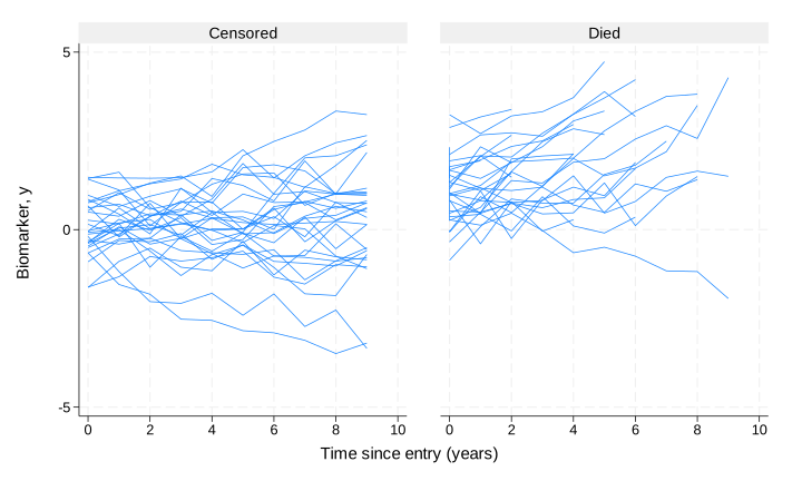

Two panels of simulated biomarker trajectories over ten years for the first 60 patients, one for those censored and one for those who died. The censored patients’ values mostly lie between about −2 and 3 and drift slowly. Those who died tend to start higher and rise, a few passing 4 before they die. — Observed biomarker trajectories for the first 60 simulated patients, by whether they died during follow-up. A patient measured only once has no line.

Those who died tend to have higher, and rising, values, which is exactly the association the joint model is built to estimate. We can fit the above joint model very simply using merlin, as follows

Stata

. merlin (y                                         /// long. outcome
>                 fp(time, powers(1 2))             /// fractional polynomial
>                 time#M2[id]@1                     /// random slope on time
>                 M1[id]@1                          /// random intercept
>                 , family(gaussian)                /// distribution
>                 timevar(time))                    /// timevar
>        (stime                                     /// survival time
>                 trt                               /// baseline trt effect
>                 EV[y]                             /// current value
>                 , family(weibull, failure(died))  /// distribution
>                 timevar(stime))                   /// timevar
>        , covariance(unstructured)                 //  VCV of random effects
variables created for model 1, component 1: _cmp_1_1_1 to _cmp_1_1_2

Fitting fixed effects model:

Fitting full model:

Iteration 0:  Log likelihood = -5529.8652  (not concave)
Iteration 1:  Log likelihood = -3903.5915
Iteration 2:  Log likelihood = -3263.3363
Iteration 3:  Log likelihood =  -3085.918
Iteration 4:  Log likelihood = -3053.7563
Iteration 5:  Log likelihood = -3052.8335
Iteration 6:  Log likelihood = -3052.8294
Iteration 7:  Log likelihood = -3052.8294

Mixed effects regression model                           Number of obs = 3,072
Log likelihood = -3052.8294
------------------------------------------------------------------------------
             | Coefficient  Std. err.      z    P>|z|     [95% conf. interval]
-------------+----------------------------------------------------------------
y:           |
      fp():1 |   .1020821   .0137042     7.45   0.000     .0752223    .1289419
      fp():2 |   .0096211   .0009942     9.68   0.000     .0076725    .0115697
 time#M2[id] |          1          .        .       .            .           .
      M1[id] |          1          .        .       .            .           .
       _cons |   .4974533   .0494716    10.06   0.000     .4004908    .5944159
  sd(resid.) |   .3516883   .0051768                      .3416869    .3619823
-------------+----------------------------------------------------------------
stime:       |
         trt |   -.538131    .140872    -3.82   0.000    -.8142351    -.262027
        EV[] |   .8182278   .0554761    14.75   0.000     .7094965     .926959
       _cons |  -3.997224   .2246973   -17.79   0.000    -4.437623   -3.556826
  log(gamma) |   .1638526   .0758806     2.16   0.031     .0151293    .3125759
-------------+----------------------------------------------------------------
id:          |
      sd(M1) |   .9471662   .0357072                      .8797045    1.019801
      sd(M2) |   .2098819   .0089231                      .1931017    .2281203
 corr(M2,M1) |   .4162753   .0491097                       .315597    .5076857
------------------------------------------------------------------------------

. estimates store value

Here, we use the EV[] element type to link the expected value of the response for the model for y, our repeatedly measured biomarker, directly to survival. Because this is a time-dependent association structure, we must specify the timevar() options to make sure merlin knows which variables represent time in both submodels. We also keep each model’s estimates with estimates store, so we can compare the fits at the end.

Looking at the results, we get an estimate of $α = 0.818$ (95% CI: 0.709, 0.927), close to the 0.8 we simulated. It’s a log hazard ratio, so $\exp (α)$ is the hazard ratio for a one-unit increase in the biomarker, at time t: the mortality rate more than doubles with each unit, a strong association. The rest of the model recovers the truth too. The treatment effect is −0.538 (we simulated −0.5); the trajectory’s intercept, linear and quadratic terms are 0.497, 0.102 and 0.0096 (0.5, 0.1 and 0.01); the residual standard deviation is 0.352 (0.35); and the random intercept and slope standard deviations and their correlation are 0.947, 0.210 and 0.416 (1, 0.2 and 0.4). The Weibull parameters are reported on the log scale, as _cons $= \log λ$ and log(gamma), and at −3.997 and 0.164 they sit close to $\log 0.02$ and $\log 1.2$ . Every estimate is within one and a half standard errors of its true value.

Note, this is a pretty simple trajectory model for our biomarker, and here we know it’s the right one, because we simulated from it. With real data we should investigate whether something more complex is required, by using more fractional polynomials or splines, but we leave that to you. Hint…it does matter (Crowther et al., 2016).

Random effects association structure

Alternatively, we can directly link individual random effects to survival, for example the random intercept,

h_{i} (t) = h_{0} (t) \exp (X_{2 i} β_{2} + α b_{0 i})

This can be fitted with merlin as follows,

Stata

. merlin (y                                         /// long. outcome
>                 fp(time, powers(1 2))             /// fractional polynomial
>                 time#M2[id]@1                     /// random slope on time
>                 M1[id]@1                          /// random intercept
>                 , family(gaussian))               /// distribution
>        (stime                                     /// survival time
>                 trt                               /// baseline trt effect
>                 M1[id]                            /// random intercept
>                 , family(weibull, failure(died))) /// distribution
>        , covariance(unstructured)                 //  VCV of random effects
variables created for model 1, component 1: _cmp_1_1_1 to _cmp_1_1_2

Fitting fixed effects model:

Fitting full model:

Iteration 0:  Log likelihood = -5529.8652  (not concave)
Iteration 1:  Log likelihood =  -3897.685
Iteration 2:  Log likelihood =  -3152.032
Iteration 3:  Log likelihood = -3116.5462
Iteration 4:  Log likelihood =  -3104.677
Iteration 5:  Log likelihood = -3104.5439
Iteration 6:  Log likelihood = -3104.5438

Mixed effects regression model                           Number of obs = 3,072
Log likelihood = -3104.5438
------------------------------------------------------------------------------
             | Coefficient  Std. err.      z    P>|z|     [95% conf. interval]
-------------+----------------------------------------------------------------
y:           |
      fp():1 |   .1001581   .0133337     7.51   0.000     .0740246    .1262917
      fp():2 |   .0084177   .0010003     8.41   0.000     .0064571    .0103783
 time#M2[id] |          1          .        .       .            .           .
      M1[id] |          1          .        .       .            .           .
       _cons |   .4999214   .0498397    10.03   0.000     .4022373    .5976055
  sd(resid.) |     .35351   .0052505                      .3433675    .3639521
-------------+----------------------------------------------------------------
stime:       |
         trt |  -.4899608   .1422347    -3.44   0.001    -.7687356   -.2111859
      M1[id] |   .9792382   .0824511    11.88   0.000      .817637    1.140839
       _cons |  -3.967902   .2424866   -16.36   0.000    -4.443167   -3.492637
  log(gamma) |    .531147   .0609584     8.71   0.000     .4116708    .6506232
-------------+----------------------------------------------------------------
id:          |
      sd(M1) |   .9543772   .0359724                      .8864138    1.027551
      sd(M2) |   .1998179   .0084037                      .1840075    .2169868
 corr(M2,M1) |   .4224694   .0498144                      .3201804    .5150214
------------------------------------------------------------------------------

. estimates store intercept

We simply include the M1[id] element in both linear predictors, and estimate a coefficient for it in the survival model. Because it’s named the same, merlin knows there are still only two random effects in this model.

Our $α$ now represents the log hazard ratio for a one-unit increase in the patient-specific deviation from the mean intercept. Given we are now using a time-independent association structure in this example, we no longer require numerical integration to calculate the cumulative hazard function, and therefore don’t need to use the timevar() option. Such an association structure provides us with computational speed gains because of this.

Here $α$ is estimated as 0.979. There’s no true value to hold it up against, because the data weren’t simulated this way, but we can compare the fits: the log-likelihood is −3104.5, against −3052.8 for the current value model, with the same number of parameters. The random intercept captures where a patient starts, but not, directly, where their trajectory goes afterwards.

Gradient or rate of change association structure

We can link the current gradient or rate of change of the biomarker directly to survival, for example

h_{i} (t) = h_{0} (t) \exp (X_{2 i} β_{2} + α m_{i}^{'} (t))

where

m_{i}^{'} (t) = \frac{\partial m_{i} (t)}{\partial t}

This can be fitted with merlin using the dEV[] element as follows

Stata

. merlin (y                                         /// long. outcome
>                 fp(time, powers(1 2))             /// fractional polynomial
>                 time#M2[id]@1                     /// random slope on time
>                 M1[id]@1                          /// random intercept
>                 , family(gaussian)                /// distribution
>                 timevar(time))                    /// timevar
>        (stime                                     /// survival time
>                 trt                               /// baseline trt effect
>                 dEV[y]                            /// current slope
>                 , family(weibull, failure(died))  /// distribution
>                 timevar(stime))                   /// timevar
>        , covariance(unstructured)                 //  VCV of random effects
variables created for model 1, component 1: _cmp_1_1_1 to _cmp_1_1_2

Fitting fixed effects model:

Fitting full model:

Iteration 0:  Log likelihood = -5529.8652  (not concave)
Iteration 1:  Log likelihood =  -5115.476  (not concave)
Iteration 2:  Log likelihood = -3769.4166
Iteration 3:  Log likelihood = -3335.5526  (not concave)
Iteration 4:  Log likelihood = -3320.6105  (not concave)
Iteration 5:  Log likelihood = -3312.4567  (not concave)
Iteration 6:  Log likelihood = -3292.7039  (not concave)
Iteration 7:  Log likelihood = -3248.9764
Iteration 8:  Log likelihood = -3231.6756  (not concave)
Iteration 9:  Log likelihood = -3207.1706
Iteration 10: Log likelihood =  -3199.296  (not concave)
Iteration 11: Log likelihood = -3180.4472
Iteration 12: Log likelihood = -3171.5671  (not concave)
Iteration 13: Log likelihood = -3128.8172
Iteration 14: Log likelihood = -3099.4339  (not concave)
Iteration 15: Log likelihood = -3090.6273
Iteration 16: Log likelihood = -3086.3452
Iteration 17: Log likelihood = -3085.2788
Iteration 18: Log likelihood = -3085.0683
Iteration 19: Log likelihood = -3085.0677
Iteration 20: Log likelihood = -3085.0677

Mixed effects regression model                           Number of obs = 3,072
Log likelihood = -3085.0677
------------------------------------------------------------------------------
             | Coefficient  Std. err.      z    P>|z|     [95% conf. interval]
-------------+----------------------------------------------------------------
y:           |
      fp():1 |   .1177228   .0143442     8.21   0.000     .0896087    .1458369
      fp():2 |    .010559   .0009881    10.69   0.000     .0086223    .0124957
 time#M2[id] |          1          .        .       .            .           .
      M1[id] |          1          .        .       .            .           .
       _cons |   .4903514   .0483002    10.15   0.000     .3956847     .585018
  sd(resid.) |   .3543486   .0052767                      .3441559    .3648432
-------------+----------------------------------------------------------------
stime:       |
         trt |  -.4945425   .1491333    -3.32   0.001    -.7868384   -.2022465
       dEV[] |    6.33697   .5499007    11.52   0.000     5.259185    7.414756
       _cons |  -5.115924   .3332225   -15.35   0.000    -5.769028   -4.462819
  log(gamma) |   .4080373   .0705323     5.79   0.000     .2697966    .5462781
-------------+----------------------------------------------------------------
id:          |
      sd(M1) |   .9224719      .0348                      .8567257    .9932634
      sd(M2) |   .2243206   .0099748                      .2055981     .244748
 corr(M2,M1) |    .483091   .0448247                       .390516    .5659935
------------------------------------------------------------------------------

. estimates store slope

where $α$ now represents the log hazard ratio for a one-unit increase in the gradient of the biomarker, at time t. You can model the biomarker over time as simply or as flexibly as you need – dEV[] will take care of the differentiation for you.

The estimate, 6.34, looks large, but a one-unit increase in the slope means the biomarker rising by one more unit per year, and we simulated random slopes with a standard deviation of only 0.2. The log-likelihood, −3085.1, is again below the current value model’s.

Cumulative association structure

We can link the cumulative value of the biomarker directly to survival, for example

h_{i} (t) = h_{0} (t) \exp (X_{2 i} β_{2} + α \int_{0}^{t} m_{i} (u) d u)

where the integral is generally approximated numerically. This can be fitted with merlin using the iEV[] element as follows

Stata

. merlin (y                                         /// long. outcome
>                 fp(time, powers(1 2))             /// fractional polynomial
>                 time#M2[id]@1                     /// random slope on time
>                 M1[id]@1                          /// random intercept
>                 , family(gaussian)                /// distribution
>                 timevar(time))                    /// timevar
>        (stime                                     /// survival time
>                 trt                               /// baseline trt effect
>                 iEV[y]                            /// current integral
>                 , family(weibull, failure(died))  /// distribution
>                 timevar(stime))                   /// timevar
>        , covariance(unstructured)                 //  VCV of random effects
variables created for model 1, component 1: _cmp_1_1_1 to _cmp_1_1_2

Fitting fixed effects model:

Fitting full model:

Iteration 0:  Log likelihood = -5529.8652  (not concave)
Iteration 1:  Log likelihood = -3906.7094
Iteration 2:  Log likelihood = -3300.2147
Iteration 3:  Log likelihood = -3126.1439
Iteration 4:  Log likelihood = -3084.1375
Iteration 5:  Log likelihood = -3083.9339
Iteration 6:  Log likelihood = -3083.9335
Iteration 7:  Log likelihood = -3083.9335

Mixed effects regression model                           Number of obs = 3,072
Log likelihood = -3083.9335
------------------------------------------------------------------------------
             | Coefficient  Std. err.      z    P>|z|     [95% conf. interval]
-------------+----------------------------------------------------------------
y:           |
      fp():1 |   .0969812   .0135247     7.17   0.000     .0704734    .1234891
      fp():2 |   .0093133   .0009974     9.34   0.000     .0073584    .0112682
 time#M2[id] |          1          .        .       .            .           .
      M1[id] |          1          .        .       .            .           .
       _cons |    .499502   .0496903    10.05   0.000     .4021107    .5968933
  sd(resid.) |    .352025   .0051889                      .3420005    .3623433
-------------+----------------------------------------------------------------
stime:       |
         trt |  -.5118491   .1406401    -3.64   0.000    -.7874986   -.2361996
       iEV[] |   .1457328   .0104965    13.88   0.000       .12516    .1663056
       _cons |  -3.004977    .206127   -14.58   0.000    -3.408979   -2.600976
  log(gamma) |  -.0178018   .0893474    -0.20   0.842    -.1929195    .1573158
-------------+----------------------------------------------------------------
id:          |
      sd(M1) |   .9516023    .035862                      .8838471    1.024552
      sd(M2) |   .2051777   .0086538                      .1888987    .2228597
 corr(M2,M1) |    .405104   .0499017                      .3029209    .4980786
------------------------------------------------------------------------------

. estimates store cumulative

where $α$ now represents the log hazard ratio for a one-unit increase in the cumulative value of the biomarker, at time t. Here it’s 0.146, with a log-likelihood of −3083.9.

Combining association structures

In many situations, more than one aspect of the biomarker may be associated with survival; for example, we can link both the current value and slope,

h_{i} (t) = h_{0} (t) \exp (X_{2 i} β_{2} + α_{1} m_{i} (t) + α_{2} m_{i}^{'} (t))

which can be estimated with,

Stata

. merlin (y                                         /// long. outcome
>                 fp(time, powers(1 2))             /// fractional polynomial
>                 time#M2[id]@1                     /// random slope on time
>                 M1[id]@1                          /// random intercept
>                 , family(gaussian)                /// distribution
>                 timevar(time))                    /// timevar
>        (stime                                     /// survival time
>                 trt                               /// baseline trt effect
>                 EV[y]                             /// current value
>                 dEV[y]                            /// current slope
>                 , family(weibull, failure(died))  /// distribution
>                 timevar(stime))                   /// timevar
>        , covariance(unstructured)                 //  VCV of random effects
variables created for model 1, component 1: _cmp_1_1_1 to _cmp_1_1_2

Fitting fixed effects model:

Fitting full model:

Iteration 0:  Log likelihood = -5529.8652  (not concave)
Iteration 1:  Log likelihood =  -5243.655  (not concave)
Iteration 2:  Log likelihood =  -4484.085  (not concave)
Iteration 3:  Log likelihood = -4317.3864  (not concave)
Iteration 4:  Log likelihood = -4100.2136  (not concave)
Iteration 5:  Log likelihood = -3890.6549  (not concave)
Iteration 6:  Log likelihood = -3617.1916  (not concave)
Iteration 7:  Log likelihood = -3581.0634  (not concave)
Iteration 8:  Log likelihood = -3484.2431
Iteration 9:  Log likelihood = -3415.3874
Iteration 10: Log likelihood = -3189.9588  (not concave)
Iteration 11: Log likelihood = -3157.7098  (not concave)
Iteration 12: Log likelihood = -3058.0137
Iteration 13: Log likelihood = -3052.0431
Iteration 14: Log likelihood = -3051.9658
Iteration 15: Log likelihood = -3051.9658

Mixed effects regression model                           Number of obs = 3,072
Log likelihood = -3051.9658
------------------------------------------------------------------------------
             | Coefficient  Std. err.      z    P>|z|     [95% conf. interval]
-------------+----------------------------------------------------------------
y:           |
      fp():1 |   .1052044   .0139875     7.52   0.000     .0777893    .1326195
      fp():2 |   .0097719   .0009989     9.78   0.000     .0078142    .0117297
 time#M2[id] |          1          .        .       .            .           .
      M1[id] |          1          .        .       .            .           .
       _cons |   .4959508   .0493976    10.04   0.000     .3991333    .5927682
  sd(resid.) |   .3516992   .0051776                      .3416963     .361995
-------------+----------------------------------------------------------------
stime:       |
         trt |  -.5367767   .1414685    -3.79   0.000    -.8140499   -.2595035
        EV[] |   .7321048   .0859468     8.52   0.000     .5636522    .9005574
       dEV[] |   1.021657   .7694236     1.33   0.184    -.4863852      2.5297
       _cons |  -4.119197   .2521989   -16.33   0.000    -4.613497   -3.624896
  log(gamma) |   .1643004   .0767566     2.14   0.032     .0138602    .3147406
-------------+----------------------------------------------------------------
id:          |
      sd(M1) |   .9454121   .0356722                      .8780185    1.017979
      sd(M2) |   .2121839   .0092653                      .1947796    .2311434
 corr(M2,M1) |   .4239698   .0488605                      .3236968     .514825
------------------------------------------------------------------------------

. estimates store combined

This time we know what to expect. We simulated from the current value alone, so once it’s in the model the slope should add nothing, and that’s what we see: the slope’s coefficient is 1.02 (95% CI: −0.49, 2.53), compatible with its true value of zero; the current value’s is 0.732 (0.564, 0.901); and the log-likelihood improves by less than one unit, from −3052.83 to −3051.97, for the extra parameter. With real data, both the value of the biomarker and where it’s going (increasing or decreasing, say) can matter, and this is how we’d find out.

Finally, we can line all five models up, using the estimates we stored along the way:

Stata

. estimates stats value intercept slope cumulative combined

Akaike's information criterion and Bayesian information criterion

-----------------------------------------------------------------------------
       Model |          N   ll(null)  ll(model)      df        AIC        BIC
-------------+---------------------------------------------------------------
       value |      3,072          .  -3052.829      11   6127.659    6193.99
   intercept |      3,072          .  -3104.544      11   6231.088   6297.419
       slope |      3,072          .  -3085.068      11   6192.135   6258.466
  cumulative |      3,072          .  -3083.933      11   6189.867   6256.198
    combined |      3,072          .  -3051.966      12   6127.932   6200.293
-----------------------------------------------------------------------------
Note: BIC uses N = number of observations. See [R] IC note.

The current value model, the one we simulated from, has the highest log-likelihood of the four single association structures, and the lowest AIC and BIC of all five models; the combined model’s extra parameter doesn’t earn its keep. Note that Stata’s BIC here counts the 3,072 rows of data, not the 400 patients, as the note under the table says.

There are numerous extensions to consider, which we will come back to in later posts. If you want to find out more, take a look at our introductory video, and at our training course on joint models.

MethodsJoint longitudinal–survival models Longitudinal data analysis

An introduction to joint modelling of longitudinal and survival data

Simulating the data

Joint model with the current value association structure

Random effects association structure

Gradient or rate of change association structure

Cumulative association structure

Combining association structures

Related at Red Door Analytics

Need this applied to your own data?