Relative survival analysis: excess mortality and net survival

Relative survival models are predominantly used in population-based cancer epidemiology (Dickman et al. 2004), where interest lies in modelling and quantifying the excess mortality in a population with a particular disease, compared to a reference population, appropriately matched on things like age, sex and calendar time. One of the benefits of the approach is that it doesn’t require accurate cause of death information.

The model

We define the total hazard at the time since diagnosis timescale, t, for the ith patient, to be $h_{i} (t)$ , with

h_{i} (t) = h_{i}^{⋆} (t) + λ_{i} (t)

where

$h_{i}^{⋆} (t)$ is the expected mortality for the ith patient, which comes from the reference population (usually life tables)
$λ_{i} (t)$ is the excess mortality for the ith patient

and we model,

λ_{i} (t) = λ_{0} (t) \exp (X_{i} β)

where $λ_{0} (t)$ is the baseline excess hazard function.

Alternatively, we can model on the (log) cumulative excess hazard scale, using the flexible parametric model of Royston and Parmar (2002), where we define the total cumulative hazard at the time since diagnosis, t, for the ith patient to be $H_{i} (t)$ , with

H_{i} (t) = H_{i}^{⋆} (t) + Λ_{i} (t)

where

$H_{i}^{⋆} (t)$ is the expected cumulative mortality for the ith patient
$Λ_{i} (t)$ is the excess cumulative mortality for the ith patient

and we model,

Λ_{i} (t) = Λ_{0} (t) \exp (X_{i} β)

where $Λ_{0} (t)$ is the baseline cumulative excess hazard function, whose log is modelled with a restricted cubic spline of log time.

The syntax

Modelling relative survival is really quite simple in terms of implementation. Our expected mortality rate is simply another variable in our dataset, which is then included in the calculation of the overall hazard function. The challenge comes with merging the expected rate file appropriately.

To turn a survival model, fitted with merlin, into a relative survival model, we simply pass the name of the variable through the bhazard() option, as follows,

merlin (depvar1 ... , family(..., failure(depvar2) bhazard(varname1)))

where depvar1 is our survival time, depvar2 is our event indicator, and varname1 is our variable which contains the expected mortality at each patient’s event time. It works with merlin’s parametric survival families, the flexible parametric rp family included.

A worked example

So let’s get to an example. This one follows Paul Dickman’s post on conditional survival, which uses colon cancer patients diagnosed 1975-94, with follow-up to 1995. We simulate a cohort shaped like that one, so we know the true net survival and can check what the model finds, and we build our own table of expected mortality rates to go with it.

First, the expected rates. In a real analysis they come from population life tables, by attained age, calendar year and sex. Ours follow a Gompertz model: the log rate is $- 10.5 + 0.1 \times age - 0.02 \times (year - 1985)$ , and 0.4 lower for women, evaluated at the middle of each one-year cell of attained age (0 to 99) and calendar year (1975 to 2000). We save them in the usual layout, one row per cell with the rate in rate, as popmort.dta.

Stata

. clear

. set seed 1975

. set obs 100                             // attained ages 0 to 99
Number of observations (_N) was 0, now 100.

. gen _age = _n - 1

. expand 26                               // calendar years 1975 to 2000
(2,500 observations created)

. bys _age : gen _year = 1974 + _n

. expand 2                                // sex: 1 male, 2 female
(2,600 observations created)

. bys _age _year : gen sex = _n

. gen rate = exp(-10.5 + 0.1*(_age + 0.5)       /// Gompertz in attained age,
>                - 0.02*(_year + 0.5 - 1985)    /// falling 2% a year,
>                - 0.4*(sex == 2))              //  lower in women

. sort _year sex _age

. save popmort, replace
(file popmort.dta not found)
file popmort.dta saved

avalon, which we use to simulate the survival times, reads a life table as a matrix with a row per cell, holding attained age, calendar year and the rate, so we make one for each sex.

Stata

. forvalues s = 1/2 {                     // an (age, year, rate) matrix per sex
  2.         mkmat _age _year rate if sex == `s', matrix(popmort`s')
  3. }

Now the patients: 10,000 of them, about half of them women, aged between 40 and 90 at diagnosis, diagnosed at a uniformly distributed date between 1975 and 1994, and followed up to the end of 1995.

Stata

. clear

. set obs 10000
Number of observations (_N) was 0, now 10,000.

. gen id = _n

. gen sex = 1 + (runiform() < 0.5)        // 1 male, 2 female

. gen age = runiform(40, 90)              // age at diagnosis

. gen yydx = runiform(1975, 1995)         // date of diagnosis, in years

. gen fu = 1996 - yydx                    // follow-up to the end of 1995

Each patient’s all-cause hazard is the sum of two parts: the expected rate for someone of their sex, attained age and calendar year, and an excess hazard due to the cancer. We give the excess hazard a Weibull form, $λ (t) = 0.2 \times 0.7 t^{- 0.3}$ , so the cumulative excess hazard is $0.2 t^{0.7}$ and the true net survival is $\exp (- 0.2 t^{0.7})$ : 0.819 at one year and 0.540 at five. avalon user simulates the all-cause survival times. chazard() gives the cumulative excess hazard, written in Mata with {t} standing for time since diagnosis; bhazard() adds the expected rate from a life table, which moves through the table as attained age, starting from age(), and calendar year, starting from year(), advance with time since diagnosis; and maxtime() censors each patient at the end of 1995. It takes one life table at a time, so we simulate everyone under each sex’s table and keep the times from their own.

Stata

. forvalues s = 1/2 {
  2.         avalon user stime`s' died`s',                   ///
>                 chazard(0.2:*{t}:^0.7)                  /// excess: Weibull
>                 bhazard(popmort`s')                     /// + expected rate,
>                 age(age) year(yydx)                     ///   at attained age
>                 maxtime(fu)                             //    and year
  3. }

. gen stime = cond(sex == 1, stime1, stime2)    // each patient's own life table

. gen died = cond(sex == 1, died1, died2)

. drop stime1 stime2 died1 died2

We stset with time since diagnosis, in years, as our timescale. There are 7,174 deaths.

Stata

. stset stime, failure(died) id(id)

Survival-time data settings

           ID variable: id
         Failure event: died!=0 & died<.
Observed time interval: (stime[_n-1], stime]
     Exit on or before: failure

--------------------------------------------------------------------------
     10,000  total observations
          0  exclusions
--------------------------------------------------------------------------
     10,000  observations remaining, representing
     10,000  subjects
      7,174  failures in single-failure-per-subject data
 46,628.872  total analysis time at risk and under observation
                                                At risk from t =         0
                                     Earliest observed entry t =         0
                                          Last observed exit t =  20.92981

We then create attained age and attained calendar time variables, in order to match appropriately when we merge in the expected rates file.

Stata

. gen _age = min(int(age + _t),99)

. gen _year = int(yydx + _t)

. sort _year sex _age

. merge m:1 _year sex _age using popmort, keep(match master)

    Result                      Number of obs
    -----------------------------------------
    Not matched                             0
    Matched                            10,000  (_merge==3)
    -----------------------------------------

Now we can fit a base case relative survival model, modelling the log cumulative excess hazard with a restricted cubic spline of log time, the Royston-Parmar model above, with three degrees of freedom.

Stata

. merlin (_t,                                     /// time since diagnosis
>         family(rp, df(3)                        /// log cumulative excess
>                failure(_d)                      ///   hazard: a spline
>                bhazard(rate)))                  //  expected rate at exit
variables created: _rcs1_1 to _rcs1_3

Fitting full model:

Iteration 0:  Log likelihood = -21086.763
Iteration 1:  Log likelihood = -17969.644
Iteration 2:  Log likelihood = -17924.207
Iteration 3:  Log likelihood = -17923.715
Iteration 4:  Log likelihood = -17923.715

Fixed effects regression model                          Number of obs = 10,000
Log likelihood = -17923.715
------------------------------------------------------------------------------
             | Coefficient  Std. err.      z    P>|z|     [95% conf. interval]
-------------+----------------------------------------------------------------
_t:          |
       _cons |  -1.000128   .0166608   -60.03   0.000    -1.032783   -.9674738
------------------------------------------------------------------------------
    Warning: Baseline spline coefficients not shown - use ml display

The rp family puts the spline on the log cumulative hazard scale, with its internal knots at quantiles of the log event times, and adding bhazard(rate) is all it takes to make it a model for the excess hazard. The spline coefficients themselves are not of much interest (ml display shows them); what the model predicts is.

We could equally put the spline on the log hazard scale, with family(loghazard) and an rcs(_t, df(3) log orthog event) element, with timevar(_t). merlin then integrates the hazard numerically, whereas on the log cumulative hazard scale the cumulative hazard is available directly.

Predicting net survival

Since we’ve fitted a relative survival model, the survival option of predict gives us net survival. We predict it at one to five years after diagnosis, and put the true net survival alongside.

Stata

. range years 1 5 5
(9,995 missing values generated)

. predict ns, survival timevar(years) ci

. gen truens = exp(-0.2*years^0.7)
(9,995 missing values generated)

. list years ns ns_lci ns_uci truens in 1/5

     +------------------------------------------------------+
     | years          ns      ns_lci      ns_uci     truens |
     |------------------------------------------------------|
  1. |     1   .81193308   .80430307   .81930002   .8187308 |
  2. |     2     .715417   .70654271   .72407793   .7225989 |
  3. |     3   .64325358   .63328395   .65303129   .6495121 |
  4. |     4   .58477798   .57410479    .5952855   .5898995 |
  5. |     5    .5355033    .5245411   .54633225   .5395424 |
     +------------------------------------------------------+

Net survival is estimated at 0.812 at one year (95% CI 0.804 to 0.819) and 0.536 at five (0.525 to 0.546), against true values of 0.819 and 0.540. The truth lies inside the 95% confidence interval at every year, though near its upper end over the first two years.

Conditional survival

We’re also often interested in conditional survival, where conditional on surviving to a timepoint $t_{0}$ , what’s the probability of surviving to time t, where $t > t_{0}$ . Let’s predict net survival conditional on surviving 1, 2 and 3 years post-diagnosis, using the ltruncated() option of predict, and compute the truth, $\exp {- 0.2 (t^{0.7} - t_{0}^{0.7})}$ , alongside.

Stata

. foreach i in 1 2 3 {
  2.         range timevar`i'  `i' 5 100
  3.         gen t`i' = `i' in 1/100
  4.         predict cs`i' , survival timevar(timevar`i') ltruncated(t`i') ci
  5.         gen true`i' = exp(-0.2*(timevar`i'^0.7 - `i'^0.7))
  6. }
(9,900 missing values generated)
(9,900 missing values generated)
(9,901 missing values generated)
note: confidence intervals calculated using Z critical values.
(9,900 missing values generated)
(9,900 missing values generated)
(9,900 missing values generated)
(9,901 missing values generated)
note: confidence intervals calculated using Z critical values.
(9,900 missing values generated)
(9,900 missing values generated)
(9,900 missing values generated)
(9,901 missing values generated)
note: confidence intervals calculated using Z critical values.
(9,900 missing values generated)

So our 5-year post-diagnosis net survival, conditional on surviving to 1 year post-diagnosis, is

Stata

. list cs1 cs1_lci cs1_uci true1 if timevar1==5

       +----------------------------------------------+
       |       cs1     cs1_lci     cs1_uci      true1 |
       |----------------------------------------------|
  100. | .65954118   .64826121   .67055692   .6589986 |
       +----------------------------------------------+

0.660 (95% CI 0.648 to 0.671), against a true value of 0.659.

Let’s plot everything, with the truth as dashed lines.

Stata

. local graph

. foreach i in 1 2 3 {
  2.         local c : word `i' of navy maroon forest_green
  3.         local graph `graph' (rarea cs`i'_lci cs`i'_uci timevar`i', ///
>                 color(`c'%30) lwidth(none))
  4.         local graph `graph' (line cs`i' timevar`i', lcolor(`c'))
  5.         local graph `graph' (line true`i' timevar`i', ///
>                 lpattern(dash) lcolor(black))
  6. }

. twoway `graph'                                          ///
>        , ytitle("Conditional net survival")             ///
>          title("Net survival conditional on"            ///
>          "surviving 1, 2, 3 years")                     ///
>          ylabel(0(0.2)1,angle(h) format(%3.1f))         ///
>          xtitle("Time since diagnosis (years)")         ///
>          xlabel(0(1)5)                                  ///
>          legend(pos(6) rows(1) order(2 "1 year"         ///
>                 5 "2 years" 8 "3 years" 3 "True"))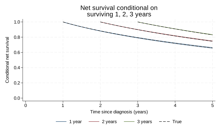

Estimated net survival conditional on surviving 1, 2 and 3 years after diagnosis, each curve starting at 1 at its conditioning time and falling to about 0.66, 0.75 and 0.83 at five years, with narrow 95% confidence bands. The true conditional net survival, drawn dashed, lies almost exactly on each estimated curve. — Net survival conditional on surviving 1, 2 and 3 years after diagnosis, with 95% confidence intervals, and the true conditional net survival (dashed).

The three estimated curves follow the truth closely, and the longer a patient has survived, the better their prospects over the rest of the five years.

Next steps

Next steps? Here’s a selection:

Flexible modelling of continuous covariates in the excess model – model age with a spline using rcs(age, df(3))
Flexible modelling of time-dependent effects: add age#rcs(_t, df(3) log orthog), alongside age and with timevar(_t), to model non-proportional hazards with splines
Hierarchical structures? Add a random intercept with M1[group]@1 in merlin
The list goes on…

MethodRelative survival

Relative survival analysis

The model

The syntax

A worked example

Predicting net survival

Conditional survival

Next steps

Need this applied to your own data?