Joint longitudinal-survival models with time-dependent effects

In this post we’ll focus on how to model time-dependent effects (non-proportional hazards), specifically within a joint longitudinal-survival model.

Now joint models are becoming commonplace in medical research, but as always, the fundamentals still matter, and indeed are often ignored. We’re going to look at how to allow both the effects of baseline covariates in the survival submodel, and the association (between the longitudinal and survival models), to vary over time. In my experience, these two assumptions are almost never considered – part of the reason is a lack of software allowing easy application and testing. Let’s remedy that.

The standard joint model

First, I recommend you take a read of this introduction to joint models, which defines the standard joint model. Let’s define it here again anyway, this time with $X_{1 i}$ and $β_{1}$ in the survival submodel and $X_{2 i} (t)$ and $β_{2}$ in the longitudinal one. Our proportional hazards submodel, assuming the current value association structure, is

h_{i} (t) = h_{0} (t) \exp (X_{1 i} β_{1} + α m_{i} (t))

with our longitudinal submodel,

y_{i} (t) = m_{i} (t) + ϵ_{i} (t)

where

m_{i} (t) = X_{2 i} (t) β_{2} + Z_{i} (t) b_{i}

and we have our normally distributed random effects,

b_{i} ~ N (0, Σ) .

Relaxing proportional hazards

Given the survival submodel is a proportional hazards model, we are making the assumption that both our hazard ratios $\exp (β_{1})$ for the covariates $X_{1 i}$ , and the hazard ratio for the effect of our biomarker, $\exp (α)$ , are constant across follow-up time. We can relax these assumptions to allow for non-proportional hazards, i.e. by modelling time-dependent effects. First we consider the following model,

h_{i} (t) = h_{0} (t) \exp (X_{1 i} β_{1} (t) + α m_{i} (t))

where if we assume $X_{1 i}$ is a binary treatment variable, we can allow its associated log hazard ratio $β_{1} (t)$ to be time-dependent, by making it a function of $\log (t)$ :

h_{i} (t) = h_{0} (t) \exp (X_{1 i} β_{1} + X_{1 i} \times β_{3} \times \log (t) + α m_{i} (t))

Simulating the data

To see these models at work, we’ll simulate data in which both proportional hazards assumptions fail, so we know what the answers should be. We generate 1,000 patients, randomise each to treatment (trt) with probability 0.5, and give each a random intercept and a random linear slope for the biomarker, independent of each other, with standard deviations 1 and 0.2.

Stata

. clear

. set seed 5813

. set obs 1000
Number of observations (_N) was 0, now 1,000.

. gen id = _n

. gen trt = runiform() > 0.5

. gen b0 = rnormal(0, 1)                  // random intercept

. gen b1 = rnormal(0, 0.2)                // random slope

Each patient’s true biomarker trajectory is

m_{i} (t) = (- 0.5 + b_{0 i}) + (0.2 + b_{1 i}) t

and we simulate their survival time from the hazard

h_{i} (t) = λ γ t^{γ - 1} \exp (X_{1 i} β_{1} + X_{1 i} \times β_{3} \times \log (t) + {α_{1} + α_{2} \times \log (t)} m_{i} (t))

which has a Weibull baseline, with $λ = 0.01$ and $γ = 2$ , and both of the time-dependent effects we’re about to model. Treatment has $β_{1} = - 1.5$ and $β_{3} = 0.6$ , so its log hazard ratio, $- 1.5 + 0.6 \log (t)$ , describes a large benefit early on that wanes over follow-up. The association between the current value of the biomarker and the hazard has $α_{1} = 1$ and $α_{2} = - 0.3$ , so it weakens over time too. We simulate with avalon, the merlin family’s simulator, giving avalon user the log of the hazard, which keeps the arithmetic stable at very small t, with the treatment effects in its covariates() and tde() options, the latter interacting treatment with tdefunction(log({t})). Anyone still alive at 10 years is censored.

Stata

. avalon user stime died,                           /// new variables
>         loghazard(log(0.01) :+ log(2)             /// log Weibull baseline
>                :+ (2-1):*log({t})                 ///
>                :+ (1 :- 0.3:*log({t}))            /// alpha1 + alpha2 log(t)
>                :* (-0.5 :+ b0                     ///   x trajectory m_i(t)
>                :+ (0.2 :+ b1):*{t}))              ///
>         covariates(trt -1.5)                      /// beta1, treatment
>         tde(trt 0.6) tdefunction(log({t}))        /// beta3, trt x log(t)
>         maxtime(10)                               //  admin. censoring
note: this hazard is close to singular at the lower limit.
      Gauss-Kronrod puts the 15-point quadrature error at  2.1e-04; the run
      used nodes() points and is better than that, but in the same regime. Raisi
> ng
      nodes() helps only slowly here -- see r(qerror).

avalon adds a note that the hazard is close to singular at the lower limit, and that more quadrature nodes help only slowly. It is a cautious check, and here a harmless one: rerunning with nodes(200) instead of the default gives the same simulated times, to within 1e-12. The biomarker is measured at entry and then annually until death or censoring, with measurement error standard deviation 0.35, and we keep one row of survival data per patient:

Stata

. expand 10
(9,000 observations created)

. bys id : gen time = _n - 1

. drop if time > stime
(2,317 observations deleted)

. gen y = -0.5 + b0 + (0.2 + b1)*time + rnormal(0, 0.35)

. bys id (time) : replace stime = . if _n > 1
(6683 real changes made, 6683 to missing)

. bys id (time) : replace died = . if _n > 1
(6,683 real changes made, 6,683 to missing)

A time-dependent treatment effect

We start with the time-dependent treatment effect model defined above, which we fit with merlin as follows,

Stata

. merlin (stime                                   /// surv. time
>                 trt                             /// treatment
>                 trt#fp(stime,pow(0))            /// treatment x log(time)
>                 EV[y]                           /// current val.
>           , family(weibull, failure(died))      /// surv. dist.
>             timevar(stime))                     /// timevar
>        (y                                       /// biomarker
>                 time                            /// fixed linear time
>                 time#M2[id]@1                   /// random linear trend
>                 M1[id]@1                        /// random intercept
>           , family(gaussian)                    /// distribution
>             timevar(time))                      //  timevar
variables created for model 1, component 2: _cmp_1_2_1 to _cmp_1_2_1

Fitting fixed effects model:

Fitting full model:

Iteration 0:  Log likelihood = -13676.766  (not concave)
Iteration 1:  Log likelihood = -8327.9648
Iteration 2:  Log likelihood = -8167.7831
Iteration 3:  Log likelihood = -8166.8128
Iteration 4:  Log likelihood =  -8166.804
Iteration 5:  Log likelihood =  -8166.804

Mixed effects regression model                           Number of obs = 7,683
Log likelihood = -8166.804
------------------------------------------------------------------------------
             | Coefficient  Std. err.      z    P>|z|     [95% conf. interval]
-------------+----------------------------------------------------------------
stime:       |
         trt |  -1.396653   .2990181    -4.67   0.000    -1.982717   -.8105879
    trt#fp() |   .4875596   .1639359     2.97   0.003     .1662512     .808868
        EV[] |   .4391132   .0265585    16.53   0.000     .3870596    .4911669
       _cons |  -4.272135   .2047191   -20.87   0.000    -4.673377   -3.870893
  log(gamma) |   .6429009     .04885    13.16   0.000     .5471567    .7386451
-------------+----------------------------------------------------------------
y:           |
        time |   .1965328   .0067827    28.98   0.000     .1832388    .2098267
 time#M2[id] |          1          .        .       .            .           .
      M1[id] |          1          .        .       .            .           .
       _cons |  -.5358883   .0335479   -15.97   0.000     -.601641   -.4701356
  sd(resid.) |   .3550421   .0033134                       .348607     .361596
-------------+----------------------------------------------------------------
id:          |
      sd(M1) |   1.034253   .0242825                      .9877382    1.082957
      sd(M2) |   .1974121   .0050856                       .187692    .2076355
------------------------------------------------------------------------------

where trt#fp(stime,pow(0)) forms an interaction between our binary treatment variable, trt, and a fractional polynomial of time, with power 0, which gives us the log of time, as desired.

Treatment’s effect does change over time. $β_{3}$ is estimated as 0.488 (95% CI: 0.166, 0.809), so the proportional hazards assumption for treatment doesn’t hold, and $β_{1}$ , the log hazard ratio at one year, when $\log (t) = 0$ , is −1.397. Both are close to the 0.6 and −1.5 we simulated. The association, 0.439, is a single number standing in for one we simulated to change over time, which brings us to the next model.

A time-dependent association

We can also relax the proportional hazards assumption on our association parameter, as follows,

h_{i} (t) = h_{0} (t) \exp (X_{1 i} β_{1} + α_{1} m_{i} (t) + α_{2} \times \log (t) \times m_{i} (t))

which can be fitted using,

Stata

. merlin (stime                                   /// surv. time
>                 trt                             /// treatment
>                 EV[y]                           /// current val.
>                 EV[y]#fp(stime,pow(0))          /// curr. val. x log(time)
>           , family(weibull, failure(died))      /// surv. dist.
>             timevar(stime))                     /// timevar
>        (y                                       /// biomarker
>                 time                            /// fixed linear time
>                 time#M2[id]@1                   /// random linear trend
>                 M1[id]@1                        /// random intercept
>           , family(gaussian)                    /// distribution
>             timevar(time))                      /// timevar
>        , technique(bfgs)                        //  optimiser
variables created for model 1, component 3: _cmp_1_3_1 to _cmp_1_3_1

Fitting fixed effects model:

Fitting full model:

Iteration 0:  Log likelihood = -13682.647
Iteration 1:  Log likelihood = -8434.2094  (backed up)
Iteration 2:  Log likelihood = -8421.6169  (backed up)
Iteration 3:  Log likelihood = -8378.3784  (backed up)
Iteration 4:  Log likelihood = -8360.8888  (backed up)
Iteration 5:  Log likelihood = -8357.8221  (backed up)
Iteration 6:  Log likelihood = -8339.6917  (backed up)
Iteration 7:  Log likelihood = -8328.9381  (backed up)
Iteration 8:  Log likelihood = -8327.7111  (backed up)
Iteration 9:  Log likelihood = -8242.7002
Iteration 10: Log likelihood = -8221.2516  (backed up)
Iteration 11: Log likelihood =  -8199.944
Iteration 12: Log likelihood = -8170.9932
Iteration 13: Log likelihood = -8169.2158
Iteration 14: Log likelihood = -8166.9374
Iteration 15: Log likelihood = -8165.4274
Iteration 16: Log likelihood = -8165.1711
Iteration 17: Log likelihood =  -8165.165
Iteration 18: Log likelihood = -8165.1643
Iteration 19: Log likelihood = -8165.1643

Mixed effects regression model                           Number of obs = 7,683
Log likelihood = -8165.1643
------------------------------------------------------------------------------
             | Coefficient  Std. err.      z    P>|z|     [95% conf. interval]
-------------+----------------------------------------------------------------
stime:       |
         trt |  -.5424831   .0774119    -7.01   0.000    -.6942076   -.3907585
        EV[] |   .8351131   .1155343     7.23   0.000       .60867    1.061556
   EV[]#fp() |  -.2147895   .0613448    -3.50   0.000    -.3350231    -.094556
       _cons |   -4.98416   .2100297   -23.73   0.000     -5.39581   -4.572509
  log(gamma) |   .8006401   .0422659    18.94   0.000     .7178005    .8834798
-------------+----------------------------------------------------------------
y:           |
        time |   .1976487   .0068008    29.06   0.000     .1843194    .2109779
 time#M2[id] |          1          .        .       .            .           .
      M1[id] |          1          .        .       .            .           .
       _cons |  -.5364873    .033536   -16.00   0.000    -.6022167    -.470758
  sd(resid.) |   .3550308    .003313                      .3485964     .361584
-------------+----------------------------------------------------------------
id:          |
      sd(M1) |    1.03385   .0242743                      .9873509    1.082538
      sd(M2) |   .1977542   .0050996                      .1880075    .2080061
------------------------------------------------------------------------------

I’ve added technique(bfgs) to this model. With these data, merlin’s default Newton–Raphson optimiser, starting from its default starting values, stalls on it in a region where the log-likelihood isn’t concave, while BFGS, which builds up its own approximation to the curvature as it goes, converges without fuss. The other models here converge with the default, so they don’t need it. If a joint model won’t converge, trying another optimiser, or better starting values, is a good first step.

The association is clearly time-dependent, with $α_{2} = - 0.215$ (95% CI: −0.335, −0.095): the log hazard ratio for a one-unit increase in the biomarker is $α_{1} = 0.835$ at one year, and it falls as time goes on. But this model has a single treatment effect, −0.542, and we already know that’s not right.

For completeness we can model non-proportional hazards in both our treatment effect and our association parameter as follows,

Stata

. merlin (stime                                   /// surv. time
>                 trt                             /// treatment
>                 trt#fp(stime,pow(0))            /// treatment x log(time)
>                 EV[y]                           /// current val.
>                 EV[y]#fp(stime,pow(0))          /// curr. val. x log(time)
>           , family(weibull, failure(died))      /// surv. dist.
>             timevar(stime))                     /// timevar
>        (y                                       /// biomarker
>                 time                            /// fixed linear time
>                 time#M2[id]@1                   /// random linear trend
>                 M1[id]@1                        /// random intercept
>           , family(gaussian)                    /// distribution
>             timevar(time))                      //  timevar
variables created for model 1, component 2: _cmp_1_2_1 to _cmp_1_2_1
variables created for model 1, component 4: _cmp_1_4_1 to _cmp_1_4_1

Fitting fixed effects model:

Fitting full model:

Iteration 0:  Log likelihood = -13676.766  (not concave)
Iteration 1:  Log likelihood =  -8313.237
Iteration 2:  Log likelihood = -8161.7871
Iteration 3:  Log likelihood = -8160.2434
Iteration 4:  Log likelihood =  -8160.237
Iteration 5:  Log likelihood =  -8160.237

Mixed effects regression model                           Number of obs = 7,683
Log likelihood = -8160.237
------------------------------------------------------------------------------
             | Coefficient  Std. err.      z    P>|z|     [95% conf. interval]
-------------+----------------------------------------------------------------
stime:       |
         trt |  -1.443317   .3058962    -4.72   0.000    -2.042862    -.843771
    trt#fp() |   .5168821   .1678584     3.08   0.002     .1878857    .8458784
        EV[] |   .8357856   .1133053     7.38   0.000     .6137113     1.05786
   EV[]#fp() |  -.2163206   .0600915    -3.60   0.000    -.3340978   -.0985435
       _cons |  -4.595266   .2357552   -19.49   0.000    -5.057337   -4.133194
  log(gamma) |   .7155279    .052049    13.75   0.000     .6135137    .8175421
-------------+----------------------------------------------------------------
y:           |
        time |   .1976233   .0068004    29.06   0.000     .1842947    .2109519
 time#M2[id] |          1          .        .       .            .           .
      M1[id] |          1          .        .       .            .           .
       _cons |  -.5365081   .0335343   -16.00   0.000     -.602234   -.4707822
  sd(resid.) |   .3550289    .003313                      .3485946     .361582
-------------+----------------------------------------------------------------
id:          |
      sd(M1) |   1.033794   .0242735                      .9872964     1.08248
      sd(M2) |   .1977549   .0050994                      .1880086    .2080064
------------------------------------------------------------------------------

This is the model we simulated from, so we can check every estimate against the truth: $β_{1} = - 1.443$ (−1.5), $β_{3} = 0.517$ (0.6), $α_{1} = 0.836$ (1) and $α_{2} = - 0.216$ (−0.3). The Weibull parameters, −4.595 and 0.716 on the log scale, sit close to $\log 0.01$ and $\log 2$ , and the longitudinal submodel recovers its intercept, −0.537 (−0.5), slope, 0.198 (0.2), residual standard deviation, 0.355 (0.35), and random-effect standard deviations, 1.034 and 0.198 (1 and 0.2). Every estimate is within two standard errors of its true value, and the log-likelihood, −8160.2, is well above those of the two models that relax only one of the assumptions, −8166.8 and −8165.2.

Numbers like $β_{1}$ and $β_{3}$ are hard to picture, so let’s plot the treatment effect over follow-up. predict’s hratio option gives the hazard ratio between the treated and placebo groups at each of 100 times from 0.1 to 10 years, which we store in tvar, with a 95% confidence interval. Treatment doesn’t act on the biomarker in this model, so the biomarker terms cancel and the hazard ratio is $\exp {β_{1} + β_{3} \log (t)}$ for everyone. I overlay the true hazard ratio, $\exp {- 1.5 + 0.6 \log (t)}$ :

Stata

. range tvar 0.1 10 100
(7,583 missing values generated)

. predict hr, hratio at1(trt 1) at2(trt 0) timevar(tvar) ci

. gen truehr = exp(-1.5 + 0.6*log(tvar))
(7,583 missing values generated)

. twoway (rarea hr_lci hr_uci tvar, color(%30))                    ///
>        (line hr tvar)                                            ///
>        (line truehr tvar, lpattern(dash))                        ///
>        , yline(1, lpattern(shortdash) lcolor(gs10))              ///
>        xtitle("Time since entry (years)")                        ///
>        ytitle("Hazard ratio, treated vs. placebo")               ///
>        ylabel(, angle(h) format(%3.1f))                          ///
>        legend(pos(6) rows(1) order(2 "Estimated" 1 "95% CI" 3 "True"))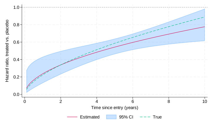

The estimated hazard ratio for treated versus placebo rises from about 0.07 at the start of follow-up to about 0.78 at ten years, with a 95% confidence band that stays below 1 throughout and ends between about 0.6 and 1.0. The true hazard ratio, dashed, rises from about 0.06 to 0.89 and lies inside the band throughout. — The hazard ratio for treated versus placebo over follow-up, from the model with both time-dependent effects, with its 95% confidence interval and the true hazard ratio we simulated from.

The benefit of treatment is large at first and wanes steadily, just as we simulated it, and the true hazard ratio lies inside the confidence band throughout. A single hazard ratio would have hidden all of that.

Other functional forms

In any of the models above, there is no restriction on what functional form we use to model each of the time-dependent effects. If a more complex form is desired, then we can use the fp() or rcs() syntax to get more flexible time functions. For example, keeping the time-dependent treatment effect, and using a higher degree fractional polynomial for the association,

Stata

. merlin (stime                                   /// surv. time
>                 trt                             /// treatment
>                 trt#fp(stime,pow(0))            /// treatment x log(time)
>                 EV[y]                           /// current val.
>                 EV[y]#fp(stime,pow(1 2))        /// curr. val. x FP2
>           , family(weibull, failure(died))      /// surv. dist.
>             timevar(stime))                     /// timevar
>        (y                                       /// biomarker
>                 time                            /// fixed linear time
>                 time#M2[id]@1                   /// random linear trend
>                 M1[id]@1                        /// random intercept
>           , family(gaussian)                    /// distribution
>             timevar(time))                      //  timevar
variables created for model 1, component 2: _cmp_1_2_1 to _cmp_1_2_1
variables created for model 1, component 4: _cmp_1_4_1 to _cmp_1_4_2

Fitting fixed effects model:

Fitting full model:

Iteration 0:  Log likelihood = -13676.766  (not concave)
Iteration 1:  Log likelihood = -8316.9715
Iteration 2:  Log likelihood = -8161.5554
Iteration 3:  Log likelihood = -8160.0667
Iteration 4:  Log likelihood =  -8160.056
Iteration 5:  Log likelihood =  -8160.056

Mixed effects regression model                           Number of obs = 7,683
Log likelihood = -8160.056
------------------------------------------------------------------------------
             | Coefficient  Std. err.      z    P>|z|     [95% conf. interval]
-------------+----------------------------------------------------------------
stime:       |
         trt |  -1.451455   .3092007    -4.69   0.000    -2.057477   -.8454327
    trt#fp() |   .5225617   .1698058     3.08   0.002     .1897485    .8553749
        EV[] |   .9261431   .1709479     5.42   0.000     .5910914    1.261195
 EV[]#fp():1 |  -.1199838   .0548098    -2.19   0.029     -.227409   -.0125585
 EV[]#fp():2 |   .0064364   .0042339     1.52   0.128    -.0018619    .0147346
       _cons |  -4.593162   .2357397   -19.48   0.000    -5.055203   -4.131121
  log(gamma) |   .7147776   .0521207    13.71   0.000     .6126229    .8169322
-------------+----------------------------------------------------------------
y:           |
        time |   .1976855   .0068014    29.07   0.000     .1843551    .2110159
 time#M2[id] |          1          .        .       .            .           .
      M1[id] |          1          .        .       .            .           .
       _cons |  -.5365232   .0335352   -16.00   0.000     -.602251   -.4707954
  sd(resid.) |   .3550294    .003313                       .348595    .3615825
-------------+----------------------------------------------------------------
id:          |
      sd(M1) |   1.033819   .0242742                      .9873206    1.082507
      sd(M2) |   .1977699   .0051002                      .1880222    .2080231
------------------------------------------------------------------------------

The true time-dependence is in $\log (t)$ , which this FP2 in $t$ and $t^{2}$ can only approximate, and the fit is essentially the same: a log-likelihood of −8160.06, against −8160.24 for the $\log (t)$ model, for one extra parameter.

Or we can use restricted cubic splines for the association,

Stata

. merlin (stime                                   /// surv. time
>                 trt                             /// treatment
>                 trt#fp(stime,pow(0))            /// treatment x log(time)
>                 EV[y]                           /// current val.
>                 EV[y]#rcs(stime, df(3) log event)   /// curr. val. x rcs
>           , family(weibull, failure(died))      /// surv. dist.
>             timevar(stime))                     /// timevar
>        (y                                       /// biomarker
>                 time                            /// fixed linear time
>                 time#M2[id]@1                   /// random linear trend
>                 M1[id]@1                        /// random intercept
>           , family(gaussian)                    /// distribution
>             timevar(time))                      //  timevar
variables created for model 1, component 2: _cmp_1_2_1 to _cmp_1_2_1
variables created for model 1, component 4: _cmp_1_4_1 to _cmp_1_4_3

Fitting fixed effects model:

Fitting full model:

Iteration 0:  Log likelihood = -13676.766  (not concave)
Iteration 1:  Log likelihood = -8312.4463
Iteration 2:  Log likelihood = -8162.0558
Iteration 3:  Log likelihood = -8160.1746
Iteration 4:  Log likelihood = -8160.1666
Iteration 5:  Log likelihood = -8160.1666

Mixed effects regression model                           Number of obs = 7,683
Log likelihood = -8160.1666
------------------------------------------------------------------------------
             | Coefficient  Std. err.      z    P>|z|     [95% conf. interval]
-------------+----------------------------------------------------------------
stime:       |
         trt |   -1.44349   .3105166    -4.65   0.000    -2.052091   -.8348887
    trt#fp() |   .5175507   .1706424     3.03   0.002     .1830978    .8520037
        EV[] |   .8311293    .151505     5.49   0.000      .534185    1.128074
EV[]#rcs():1 |  -.1821175   .1858561    -0.98   0.327    -.5463887    .1821537
EV[]#rcs():2 |    .239172   .6469247     0.37   0.712    -1.028777    1.507121
EV[]#rcs():3 |  -.4792693   1.288014    -0.37   0.710     -3.00373    2.045191
       _cons |  -4.598089   .2382521   -19.30   0.000    -5.065055   -4.131123
  log(gamma) |   .7160394    .052668    13.60   0.000     .6128119    .8192668
-------------+----------------------------------------------------------------
y:           |
        time |   .1976547   .0068012    29.06   0.000     .1843246    .2109849
 time#M2[id] |          1          .        .       .            .           .
      M1[id] |          1          .        .       .            .           .
       _cons |  -.5365157   .0335343   -16.00   0.000    -.6022417   -.4707896
  sd(resid.) |   .3550295    .003313                      .3485951    .3615826
-------------+----------------------------------------------------------------
id:          |
      sd(M1) |    1.03379   .0242739                      .9872918    1.082477
      sd(M2) |   .1977636   .0050999                      .1880164    .2080161
------------------------------------------------------------------------------

where rcs(stime, df(3) log event) creates a restricted cubic spline of log time, with 3 degrees of freedom, with internal knots based on centiles of the observed event distribution. Phew. The first spline term is log time itself, so this model contains the one we simulated from, with true coefficients of 1 on EV[], −0.3 on the first spline term and zero on the other two. The estimates, 0.831, −0.182, 0.239 and −0.479, are all within about one standard error of those values, and the two extra parameters improve the log-likelihood by less than 0.1, from −8160.24 to −8160.17, so there’s nothing to be gained over $\log (t)$ here.

As always, there’s a lot more merlin can do, but hopefully this serves as a taster of modelling non-proportional hazards within a joint model framework.

MethodJoint longitudinal–survival models

Joint longitudinal-survival models with time-dependent effects

The standard joint model

Relaxing proportional hazards

Simulating the data

A time-dependent treatment effect

A time-dependent association

Other functional forms

Need this applied to your own data?