Joint longitudinal and competing risks models

This post takes a look at an extension of the standard joint longitudinal-survival model, which is to incorporate competing risks. Let’s start by formally defining the model.

The model

We will assume a continuous longitudinal outcome,

where

and ${ϵ}_i(t)$ is our normally distributed residual variability. We call $m_i(t)$ our trajectory function, representing the true underlying value of the continuous outcome at time t, which is a function of fixed and random effects with associated design matrices, $X_{1i}(t)$ and $Z_i(t)$, and coefficients, ${\beta }_1$ and $b_i$. We assume normally distributed random effects,

We then have K competing events, each of which can be dependent on some (or many) aspects of the biomarker trajectory function, $m_i(t)$. To keep things simple, we will work with the current value association structure. So, for the kth competing risk we parameterise the cause-specific hazard function as,

where ${\alpha }_k$ is the log hazard ratio for the kth cause, for a one-unit increase in the biomarker, at time t. Each competing event can be modelled however we like, with different baseline hazard functions, and with different covariate effects. Of course, we can also have different or additional association structures for each event.

Simulating the data

To illustrate, we’re going to show you how to simulate data from a joint longitudinal and competing risks model, with two competing risks, representing death from cancer and death from other causes, and then show how to fit the true model using merlin.

Let’s assume a simple random intercept and random linear trend for the biomarker trajectory, i.e.

We start by setting a seed (as we always should), generate a sample of 500 patients, and create an id variable.

. clear

. set seed 7254

. set obs 500
Number of observations (_N) was 0, now 500.

. gen id = _n

Next we generate our subject-specific random effects, for the intercept and slope, with standard deviations of 1 and 0.2. We need a single draw from each distribution, per patient. We’re assuming the random effects are independent, but that’s easily adapted using drawnorm. We also generate a treatment group indicator, assigning to each arm with 50% probability.

. gen b0 = rnormal(0,1)

. gen b1 = rnormal(0,0.2)

. gen trt = runiform()>0.5

Simulating the cause-specific event times

Now we simulate cause-specific event times, using avalon msm, the multi-state subcommand of avalon, the merlin family’s simulator. Simulating joint longitudinal-survival data is not the easiest of tasks mathematically, but with avalon it’s pretty simple (Crowther, 2022, describes the method as it was first implemented, in its predecessor survsim). We simply specify our cause-specific hazard functions, and avalon does the hard work (numerical integration nested within root-finding), details in Crowther and Lambert (2013).

We specify our baseline distribution parameters, the scale and shape, for Weibull baseline hazards for causes one and two, and an administrative censoring time of 5 years. We also specify a treatment effect with a log hazard ratio of −0.5 on cause 1 and −0.2 on cause 2. Putting this all together in user-defined functions in avalon msm, simulating under the current value association structure, defining ${\alpha }_1=0.5$ and ${\alpha }_2=-0.3$, we get,

. //cause one
. local maxt 5

. local l1 0.1

. local g1 1.2

. local l2 0.05

. local g2 1.5

. avalon msm stime state event,                   /// new variables
>         hazard1(                                /// cause 1 (cancer)
>                 user(`l1':*`g1':*{t}:^(`g1'-1)  /// user-defined function
>                      :* exp(0.5                 /// biomarker
>                      :* (b0 :+ (0.1:+b1):*{t})  ///   trajectory
>                      ))                         ///
>                 covariates(trt -0.5))           /// treatment effect (PH)
>         hazard2(                                /// cause 2 (other)
>                 user(`l2':*`g2':*{t}:^(`g2'-1)  /// user-defined function
>                      :* exp( -0.3 :*            /// biomarker
>                      (b0 :+ (0.1:+b1):*{t})     ///   trajectory
>                      ))                         ///
>                 covariates(trt -0.2))           /// treatment effect (PH)
>         maxtime(`maxt')                         //  admin. censoring

Now avalon is designed for many situations, such as allowing you to define your own custom hazard functions, which can depend on time…or a time-dependent biomarker trajectory. It also provides a general framework to simulate from competing risks and multi-state survival models. In this example, we are simulating from an all-cause hazard function, which is a function of two cause-specific hazards, each of which depends on a time-dependent biomarker trajectory. That’s a mouthful. Ok, so to start we define some new variable stubs, to contain the variables that avalon msm will create. stime* will contain the start and stop times for each transition, state* will contain the start and stop states, and event* will be flag indicator variables for whether an event/transition occurred, or an observation was censored.

Let’s see what we created:

. list id trt stime* state* event* if _n<=5

     +----------------------------------------------------------+
     | id   trt   stime0      stime1   state0   state1   event1 |
     |----------------------------------------------------------|
  1. |  1     0        0   2.4400787        1        2        1 |
  2. |  2     0        0   3.1501589        1        2        1 |
  3. |  3     1        0   1.7629374        1        3        1 |
  4. |  4     0        0           5        1        1        0 |
  5. |  5     0        0    1.432066        1        3        1 |
     +----------------------------------------------------------+

So all observations started in state 1 (state0 is a 1) at time 0 (stime0 is 0). Observation 4 was censored (event1 is a 0) at 5 years, observations 1 and 2 moved to state 2 at various times, i.e. died due to cancer, and observations 3 and 5 died from other causes (state1 is a 3), at 1.763 and 1.432 years. As it’s a competing risks situation (which is what avalon msm assumes unless you specify your own transition matrix), then observations can only go from the starting state 1 to states 2 or 3, corresponding to hazard1 and hazard2, respectively.

All that’s left to do is to create our cause-specific event indicators, which we will need in our estimation step. We’ll then drop variables we no longer need.

. gen byte cancer = state1==2

. gen byte other = state1==3

. drop stime0 state0 state1 event1

Generating the biomarker measurements

Now we’re all done with the competing risk outcomes. Onto the biomarker.

Let’s assume a setting where our biomarker is recorded at baseline, and then annually, so each patient can have up to five measurements. The easiest thing to do is to expand our dataset, by creating replicants of each row, and then drop any observations which occur after each patient’s event/censoring time.

. expand 5
(2,000 observations created)

. bys id : gen time = _n-1

. drop if time>stime1
(713 observations deleted)

We generate our observed longitudinal biomarker measurements from the true model above,

. gen xb = b0 + 0.1 * time + b1 * time

. gen y = rnormal(xb,0.5)                 //measurement error

It’s easiest to work in wide format for merlin (I mean in terms of the outcomes, they are side by side, but within each outcome the observations are in long format), so for the competing risks outcomes we need to have only a single row of data per patient, so we replace the repeated event times and event indicators with missing values.

. bys id (time) : replace stime1 = . if _n>1
(1287 real changes made, 1287 to missing)

. bys id (time) : replace cancer = . if _n>1
(1,287 real changes made, 1,287 to missing)

. bys id (time) : replace other = . if _n>1
(1,287 real changes made, 1,287 to missing)

Fitting the model

We’re now all set up to fit our data-generating, true model, with merlin:

. merlin (y                       /// biomarker outcome
>           time                  /// fixed linear time
>           time#M2[id]@1         /// random slope on linear time
>           M1[id]@1,             /// random intercept
>           family(gaussian)      /// distribution
>           timevar(time))        /// variable representing time
>        (stime1                  /// survival time
>           trt                   /// baseline treatment
>           EV[y],                /// expected value of biomarker
>           family(weibull,       /// distribution
>                failure(cancer)) /// cause-specific event indicator
>           timevar(stime1))      /// timevar
>        (stime1                  /// survival time
>           trt                   /// baseline treatment
>           EV[y],                /// expected value of biomarker
>           family(weibull,       /// distribution
>                failure(other))  /// cause-specific event indicator
>           timevar(stime1))      //  timevar

Fitting fixed effects model:

Fitting full model:

Iteration 0:  Log likelihood = -3758.8927
Iteration 1:  Log likelihood = -3223.8211
Iteration 2:  Log likelihood =  -3186.752
Iteration 3:  Log likelihood = -3186.0523
Iteration 4:  Log likelihood = -3186.0519
Iteration 5:  Log likelihood = -3186.0519

Mixed effects regression model                           Number of obs = 1,787
Log likelihood = -3186.0519
------------------------------------------------------------------------------
             | Coefficient  Std. err.      z    P>|z|     [95% conf. interval]
-------------+----------------------------------------------------------------
y:           |
        time |   .1288292   .0151716     8.49   0.000     .0990935     .158565
 time#M2[id] |          1          .        .       .            .           .
      M1[id] |          1          .        .       .            .           .
       _cons |   .0499435   .0496237     1.01   0.314    -.0473172    .1472042
  sd(resid.) |   .5067381   .0115473                      .4846037    .5298835
-------------+----------------------------------------------------------------
stime1:      |
         trt |  -.6467427   .1383104    -4.68   0.000    -.9178261   -.3756594
        EV[] |   .4945694   .0682039     7.25   0.000     .3608922    .6282465
       _cons |  -2.197094   .1375495   -15.97   0.000    -2.466686   -1.927502
  log(gamma) |   .1766552    .062348     2.83   0.005     .0544553     .298855
-------------+----------------------------------------------------------------
stime1:      |
         trt |   .0103315    .178023     0.06   0.954    -.3385871    .3592501
        EV[] |  -.3310918    .083776    -3.95   0.000    -.4952897   -.1668938
       _cons |  -2.997267   .1951288   -15.36   0.000    -3.379713   -2.614822
  log(gamma) |   .3028744   .0776663     3.90   0.000     .1506513    .4550975
-------------+----------------------------------------------------------------
id:          |
      sd(M1) |   1.025342    .036774                      .9557414    1.100011
      sd(M2) |   .2067488   .0142555                      .1806142    .2366651
------------------------------------------------------------------------------

which we would say is rather elegantly simple to specify for such a complex model…you may disagree. We’re using the EV[y] element type to link the current value of the biomarker to each cause-specific hazard model, making sure to specify the timevar() options, so time is correctly handled. We can use stime1 as our outcome in both survival models but simply use the cause-specific event indicators so we get the correct contributions to the likelihood. It’s important to note that competing risks models with exactly observed event data, can generally be fitted either with a stacked dataset, or separately, with cumulative incidence predictions calculated post-estimation – this is not true in such a joint model, since the biomarker model appears in both cause-specific hazard functions, and hence must be estimated simultaneously.

The model fits beautifully…phew, in five iterations. Because we simulated the data, we know what it should find. For death from cancer, the log hazard ratio for treatment is −0.647 (we simulated −0.5) and the association with the current value of the biomarker is 0.495 (0.5). For death from other causes they are 0.010 (−0.2) and −0.331 (−0.3). The random intercept and slope standard deviations are 1.03 and 0.21 (1 and 0.2), and the residual standard deviation is 0.51 (0.5). Every estimate is within two standard errors of the truth; the furthest is the mean slope of the biomarker, 0.129 against 0.1.

Predicting cumulative incidence

Now we have our fitted model, generally of most interest within a competing risks analysis is both the cause-specific hazard ratios, which we get from our results table, and estimates of the cause-specific cumulative incidence functions.

We use merlin‘s predict engine to help us with such things. When predicting something which depends on time, it’s often much easier to specify a timevar(), which contains timepoints at which to predict at, which subsequently makes plotting much easier. So now we’ll generate a new variable tvar which will contain time points between 0 and 5, at 500 equally spaced points.

. range tvar 0 5 500
(1,287 missing values generated)

Let’s now predict each cause-specific cumulative incidence function, in particular, we’ll predict marginal CIFs (integrating out the random effects), so we can interpret them as population-average predictions. We’ll also use the at() option so we can investigate the effect of treatment.

. predict cif1, cif marginal outcome(2) at(trt 0) timevar(tvar)
(1287 missing values generated)

. predict cif2, cif marginal outcome(2) at(trt 1) timevar(tvar)
(1287 missing values generated)

. predict cif3, cif marginal outcome(3) at(trt 0) timevar(tvar)
(1287 missing values generated)

. predict cif4, cif marginal outcome(3) at(trt 1) timevar(tvar)
(1287 missing values generated)

Stacked CIF plots

For plotting purposes, we often create stacked plots of CIFs, and one way to do this is to add them appropriately together to draw the area under the curve, and then overlay one of the CIFs.

. gen totalcif1 = cif1 + cif3
(1,287 missing values generated)

. gen totalcif2 = cif2 + cif4
(1,287 missing values generated)

We now plot the stacked, marginal CIFs for those in the placebo group and those in the treated group, side by side. Stacking the two groups’ predictions and using twoway’s by() option draws both panels with one shared legend, and needs nothing beyond Stata itself:

. preserve

. keep tvar cif1-cif4 totalcif1 totalcif2

. keep if tvar < .
(1,287 observations deleted)

. expand 2
(500 observations created)

. bys tvar : gen byte group = _n - 1           // 0 placebo, 1 treated

. gen top    = cond(group, totalcif2, totalcif1)

. gen bottom = cond(group, cif4, cif3)

. label define group 0 "Placebo group" 1 "Treated group"

. label values group group

. twoway (area top tvar) (area bottom tvar),                          ///
>         by(group, note("") legend(pos(6)))                           ///
>         xtitle("Time since entry") ytitle("Cumulative incidence")    ///
>         legend(cols(1) order(1 "Prob. of death due to cancer"        ///
>                 2 "Prob. of death due to other causes"))             ///
>         xlabel(0(1)5) ylabel(0(0.1)1, angle(h) format(%2.1f))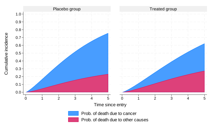

The treatment difference

We can directly quantify the impact of treatment on a CIF by predicting the difference — here for death due to cancer, outcome(2) — using the cifdifference option, combined with at1() and at2() statements.

. predict diffcif, cifdifference marginal outcome(2)       ///
>                  at1(trt 1) at2(trt 0) timevar(tvar)     ///
>                  ci

. twoway  (rarea diffcif_lci diffcif_uci tvar)                    ///
>         (line diffcif tvar)                                     ///
>         , xtitle("Time since entry")                            ///
>         ytitle("Difference in cumulative incidence")            ///
>         title("CIF({it:t} | treated) - CIF({it:t} | placebo)")  ///
>         ylabel(,angle(h) format(%3.2f))                         ///
>         legend(pos(6) rows(1) order(2 "Diff. in CIF" 1 "95% confidence interva
> l"))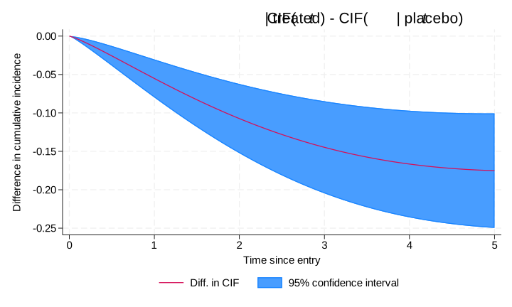

We’ll leave it there for now. The joint model we’ve covered is an introductory example in the competing risks setting. Given merlin‘s capabilities, it’s rather simple to extend to using other associations structures, such as the rate of change (dEV[y]) or the integral (iEV[y]) of the trajectory function, and to use different distributions for each cause-specific hazard model…the list of extensions goes on.

Happy joint modelling.

MethodsJoint longitudinal–survival models Competing risks Simulation studies