Relative survival analysis

Relative survival models are predominantly used in population based cancer epidemiology (Dickman et al. 2004), where interest lies in modelling and quantifying the excess mortality in a population with a particular disease, compared to a reference population, appropriately matched on things like age, gender and calendar time. One of the benefits of the approach is that it doesn’t require accurate cause of death information.

We therefore define the total hazard at the time since diagnosis timescale, t, for the ith patient, to be \(h_{i}(t)\), with

$$h_{i}(t) = h_{i}^{\star}(t) + \lambda_{i}(t)$$

where

• \(h_{i}^{\star}(t)\) is the expected mortality for the ith patient, which comes from the reference population (usually life-tables)
• \(\lambda_{i}(t)\) is the excess mortality for the ith patient

and we model,

$$\lambda_{i}(t) = \lambda_{0}(t) \exp(X_{i} \beta)$$

where \(\lambda_{0}(t)\) is the baseline hazard function.

Alternatively, we can model on the (log) cumulative excess hazard scale, using the flexible parametric model of Royston and Parmar (2002), where we define the total cumulative hazard at the time since diagnosis, t, for the ith patient to be \(H_{i}(t)\), with

$$H_{i}(t) = H_{i}^{\star}(t) + \Lambda_{i}(t)$$

where

• \(H_{i}^{\star}(t)\) is the expected cumulative mortality for the ith patient
• \(\Lambda_{i}(t)\) is the excess cumulative mortality for the ith patient

and we model,

$$\Lambda_{i}(t) = \Lambda_{0}(t)\exp (X_{i}\beta)$$

where \(\Lambda_{0}(t)\) is the baseline cumulative hazard function, modeled with restricted cubic splines.

In terms of modelling relative survival, it really is quite simple in terms of implementation. Our expected mortality rate is simply another variable in our dataset, which is then included in the calculation of the overall hazard function. The challenge comes with merging the expected rate file appropriately.

To turn a survival model, fitted with merlin, into a relative survival model, we simply pass the name of the variable through the bhazard() option, as follows,

merlin (depvar1 ... , family(..., failure(depvar2) bhazard(varname1)))

where depvar1 is our survival time, depvar2 is our event indicator, and varname1 is our variable which contains the expected mortality at each patient’s event time. It’s even easier with stmerlin,

stmerlin ... , distribution(...) bhazard(varname1)

So let’s get to an example. This one is based entirely on Paul Dickman’s post available here. We use a dataset of colon cancer patients, diagnosed 1975-94, with follow-up to 1995. We stset with time since diagnosis as our timescale, scaling it into years.

. use https://pauldickman.com/data/colon.dta, clear
(Colon carcinoma, diagnosed 1975-94, follow-up to 1995)

. stset exit, origin(dx) fail(status==1 2) id(id) scale(365.24)

Survival-time data settings

           ID variable: id
         Failure event: status==1 2
Observed time interval: (exit[_n-1], exit]
     Exit on or before: failure
     Time for analysis: (time-origin)/365.24
                Origin: time dx

--------------------------------------------------------------------------
     15,564  total observations
          0  exclusions
--------------------------------------------------------------------------
     15,564  observations remaining, representing
     15,564  subjects
     10,918  failures in single-failure-per-subject data
 58,464.051  total analysis time at risk and under observation
                                                At risk from t =         0
                                     Earliest observed entry t =         0
                                          Last observed exit t =  20.96156

We then create attained age and attained calendar time variables, in order to match appropriately when we merge in the expected rates file.

. gen _age = min(int(age + _t),99)

. gen _year = int(yydx + _t)

. sort _year sex _age

. merge m:1 _year sex _age using "http://pauldickman.com/data/popmort", keep(match master
> )

    Result                      Number of obs
    -----------------------------------------
    Not matched                             0
    Matched                            15,564  (_merge==3)
    -----------------------------------------

Now we can fit a base case relative survival model, modelling the excess mortality using restricted cubic splines on the log hazard scale.

. stmerlin, dist(rcs) df(3) bhazard(rate) 
variables created for model 1, component 1: _cmp_1_1_1 to _cmp_1_1_3

Fitting full model:

Iteration 0:   log likelihood = -57733.702  
Iteration 1:   log likelihood = -23599.411  
Iteration 2:   log likelihood =  -23491.65  
Iteration 3:   log likelihood =  -22316.87  
Iteration 4:   log likelihood = -22311.661  
Iteration 5:   log likelihood = -22311.645  
Iteration 6:   log likelihood = -22311.645  

Survival model                                          Number of obs = 15,564
Log likelihood = -22311.645
------------------------------------------------------------------------------
             | Coefficient  Std. err.      z    P>|z|     [95% conf. interval]
-------------+----------------------------------------------------------------
_t:          |            
     rcs():1 |   -1.27194    .026982   -47.14   0.000    -1.324824   -1.219056
     rcs():2 |   .4148327   .0233572    17.76   0.000     .3690534    .4606119
     rcs():3 |  -.0385967   .0159872    -2.41   0.016    -.0699309   -.0072624
       _cons |  -2.280201   .0245017   -93.06   0.000    -2.328223   -2.232178
------------------------------------------------------------------------------

Since we’ve estimated a relative survival model, we will be estimating net survival, when using the survival option of the predict function.

. predict s, survival ci
note: confidence intervals calculated using Z critical values.

We’re also often interested in conditional survival, where conditional on surviving to a timepoint \(t_{0}\), what’s the probability of surviving at time t, where \(t > t_{0}.\) Let’s predict net survival conditional on surviving 1, 2 and 3 years post-diagnosis.

. foreach i in 1 2 3 {
  2.         range timevar`i'  `i' 5 100
  3.         gen t`i' = `i' in 1/100
  4.         predict cs`i' , survival timevar(timevar`i') ltruncated(t`i') ci
  5. }

So our 5 year post-diagnosis net survival, conditional on surviving to 1 year post-diagnosis, is

. list cs1 cs1_lci cs1_uci if timevar1==5

       +-----------------------------------+
       |       cs1     cs1_lci     cs1_uci |
       |-----------------------------------|
  100. | .71140919   .70105202   .72148233 |
       +-----------------------------------+

Let’s plot everything.

. foreach i in 1 2 3 {
  2.         local graph `graph'  (rarea cs`i'_lci cs`i'_uci timevar`i', sort) 
  3.         local graph `graph'  (line cs`i' timevar`i', sort lpattern(solid))
  4. }

. 
. twoway `graph'                                          ///
>        , ytitle("Conditional relative survival")        ///
>          title("Relative survival conditional on"       ///
>          "surviving 1, 2, 3 years")                     ///
>          ylabel(0(0.2)1,angle(h) format(%3.1f))         ///
>          xtitle("Time since diagnosis (years)")         ///
>          xlabel(0(1)5) legend(off) ysize(8) xsize(11)   ///
>          name(condsurv1, replace)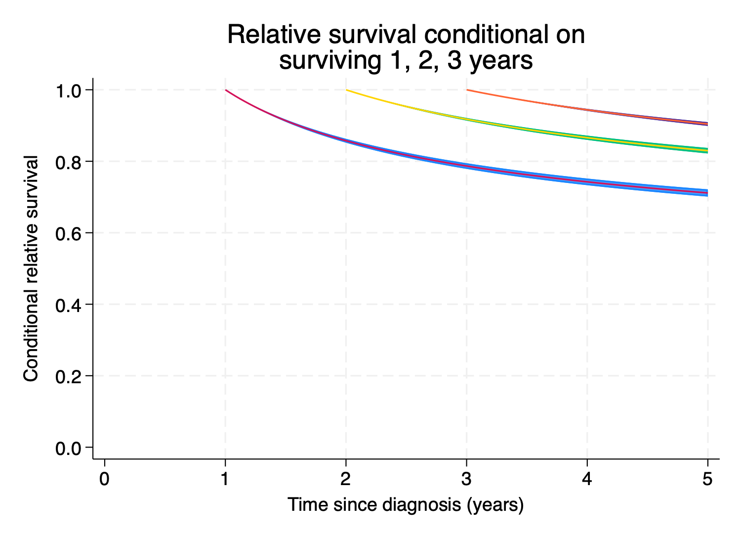

Lovely.

Next steps? Here’s a selection:

• Flexible modelling of continuous covariates in the excess model – model age with a spline using rcs(age, df(3))
• Flexible modelling of time-dependent effects: add tvc(age) dftvc(3) to model non-proportional hazards with splines in stmerlin
• Hierarchical structures? Add a random intercept with M1[group]@1 in merlin
• The list goes on…