
The headlines:
predictmsnow supports the Cox model as a transition model, estimated using
merlinorstmerlin- Predictions from a multi-state Cox model are implemented using a
simulation approach - Supported predictions from a multi-state Cox model include transition
probabilities,probability, and length of stay,los
Let’s take a look at what we can now do with multistate and in particular,
the predictms command.
We’ll use the breast cancer dataset that is included in the multistate package. We load the data,
. use http://fmwww.bc.edu/repec/bocode/m/multistate_example, clear
(Rotterdam breast cancer data, truncated at 10 years)
which comes in wide format,
. list pid rf rfi os osi if pid==1 | pid==1371, sepby(pid) noobs
  +-------------------------------------+
  |  pid     rf   rfi     os        osi |
  |-------------------------------------|
  |    1   59.1     0   59.1      alive |
  |-------------------------------------|
  | 1371   16.6     1   24.3   deceased |
  +-------------------------------------+
where pid is our patient identifier, rf contains the time of recurrence, rfi the recurrence event indicator, os overall survival time and osi our survival indicator. We can use msset to reshape our wide dataset into the stacked format, with a row for each transition of which a patient is at risk for.
. msset, id(pid) states(rfi osi) times(rf os)msset creates internal variables for use in subsequent analyses, similar to stset,
. list pid _start _stop _from _to _status _trans if pid==1 | pid==1371, noobs
  +---------------------------------------------------------------+
  |  pid      _start       _stop   _from   _to   _status   _trans |
  |---------------------------------------------------------------|
  |    1           0   59.104721       1     2         0        1 |
  |    1           0   59.104721       1     3         0        2 |
  | 1371           0   16.558521       1     2         1        1 |
  | 1371           0   16.558521       1     3         0        2 |
  | 1371   16.558521   24.344969       2     3         1        3 |
  +---------------------------------------------------------------+
and also returns a default transition matrix, if one was not provided. We need to store this for later use. In this case it’s the illness-death transition matrix, as it will assume an upper triangular transition matrix, with a common initial state.
. mat tmat = r(transmatrix)
. mat list tmat
tmat[3,3]
               to:    to:    to:
            start    rfi    osi
from:start      .      1      2
  from:rfi      .      .      3
  from:osi      .      .      .
We can now stset our dataset, using the msset created variables,
. stset _stop, enter(_start) failure(_status==1) scale(12)

Survival-time data settings

         Failure event: _status==1
Observed time interval: (0, _stop]
     Enter on or after: time _start
     Exit on or before: failure
     Time for analysis: time/12

--------------------------------------------------------------------------
      7,482  total observations
          0  exclusions
--------------------------------------------------------------------------
      7,482  observations remaining, representing
      2,790  failures in single-record/single-failure data
 38,474.539  total analysis time at risk and under observation
                                                At risk from t =         0
                                     Earliest observed entry t =         0
                                          Last observed exit t =  19.28268
We also changed the timescale from months into years by using scale(12). Tumour size at diagnosis, size, is a three-level factor variable, which we now create dummy indicator variables by,
. tab size, gen(sz)

     Tumour |
    size, 3 |
classes (t) |      Freq.     Percent        Cum.
------------+-----------------------------------
    <=20 mm |      3,339       44.63       44.63
  >20-50mmm |      3,327       44.47       89.09
     >50 mm |        816       10.91      100.00
------------+-----------------------------------
      Total |      7,482      100.00
Neither merlin or predictms support factor variables so you must create your own dummies. We can now fit our multi-state model, in this case fitting transition-specific Cox models. For transition 1,
. stmerlin age sz2 sz3 nodes pr_1 hormon if _trans==1, dist(cox)
Obtaining initial values

Fitting full model:

Iteration 0:   log likelihood = -11210.638
Iteration 1:   log likelihood = -11209.949
Iteration 2:   log likelihood = -11209.948

Survival model                                           Number of obs = 2,982
Log likelihood = -11209.948
------------------------------------------------------------------------------
             | Coefficient  Std. err.      z    P>|z|     [95% conf. interval]
-------------+----------------------------------------------------------------
_t:          |
         age |  -.0065188   .0020942    -3.11   0.002    -.0106234   -.0024141
         sz2 |   .3699927   .0579848     6.38   0.000     .2563447    .4836407
         sz3 |   .6465575   .0871242     7.42   0.000     .4757972    .8173178
       nodes |   .0787774   .0045086    17.47   0.000     .0699407    .0876141
        pr_1 |  -.0440715   .0115572    -3.81   0.000    -.0667232   -.0214198
      hormon |  -.0545278   .0823277    -0.66   0.508    -.2158871    .1068315
------------------------------------------------------------------------------

. estimates store m1
Note I use stmerlin, which is a wrapper for the more complex merlin command, but it uses the st variables created by stset so is much more convenient for use when fitting standard survival models. We can reassure ourselves that stmerlin‘s Cox model agrees with official Stata’s stcox,
. stcox age sz2 sz3 nodes pr_1 hormon if _trans==1

         Failure _d: _status==1
   Analysis time _t: _stop/12
  Enter on or after: time _start

Iteration 0:   log likelihood = -11429.625
Iteration 1:   log likelihood =   -11225.2
Iteration 2:   log likelihood = -11209.961
Iteration 3:   log likelihood = -11209.948
Refining estimates:
Iteration 0:   log likelihood = -11209.948

Cox regression with Breslow method for ties

No. of subjects =       2,982                           Number of obs =  2,982
No. of failures =       1,518
Time at risk    = 17,203.8001
                                                        LR chi2(6)    = 439.35
Log likelihood = -11209.948                             Prob > chi2   = 0.0000

------------------------------------------------------------------------------
          _t | Haz. ratio   Std. err.      z    P>|z|     [95% conf. interval]
-------------+----------------------------------------------------------------
         age |   .9935024   .0020806    -3.11   0.002     .9894329    .9975888
         sz2 |   1.447724   .0839459     6.38   0.000     1.292198    1.621969
         sz3 |   1.908958   .1663164     7.42   0.000     1.609296    2.264418
       nodes |   1.081963   .0048782    17.47   0.000     1.072445    1.091567
        pr_1 |   .9568855   .0110589    -3.81   0.000     .9354541    .9788079
      hormon |   .9469315   .0779587    -0.66   0.508     .8058257    1.112746
------------------------------------------------------------------------------
which indeed it does. Phew. For transition 2,
. stmerlin age sz2 sz3 nodes pr_1 hormon if _trans==2, dist(cox)
Obtaining initial values

Fitting full model:

Iteration 0:   log likelihood = -1187.0791
Iteration 1:   log likelihood = -1186.9616
Iteration 2:   log likelihood = -1186.9616

Survival model                                           Number of obs = 2,982
Log likelihood = -1186.9616
------------------------------------------------------------------------------
             | Coefficient  Std. err.      z    P>|z|     [95% conf. interval]
-------------+----------------------------------------------------------------
_t:          |
         age |   .1276223   .0080824    15.79   0.000      .111781    .1434635
         sz2 |   .1803381   .1613346     1.12   0.264     -.135872    .4965482
         sz3 |   .4201997   .2333692     1.80   0.072    -.0371956     .877595
       nodes |   .0438643   .0184724     2.37   0.018     .0076591    .0800694
        pr_1 |   .0306077   .0335758     0.91   0.362    -.0351997    .0964151
      hormon |  -.0934567   .2313061    -0.40   0.686    -.5468083    .3598949
------------------------------------------------------------------------------

. estimates store m2
and for transition 3,
. stmerlin age sz2 sz3 nodes pr_1 hormon if _trans==3, dist(cox)
note; a delayed entry model is being fitted
Obtaining initial values

Fitting full model:

Iteration 0:   log likelihood = -6277.4464
Iteration 1:   log likelihood = -6277.4409
Iteration 2:   log likelihood = -6277.4409

Survival model                                           Number of obs = 1,518
Log likelihood = -6277.4409
------------------------------------------------------------------------------
             | Coefficient  Std. err.      z    P>|z|     [95% conf. interval]
-------------+----------------------------------------------------------------
_t:          |
         age |   .0047152   .0024199     1.95   0.051    -.0000277    .0094581
         sz2 |   .1612421   .0712509     2.26   0.024      .021593    .3008913
         sz3 |   .3141532   .0992226     3.17   0.002     .1196805     .508626
       nodes |   .0288918   .0057254     5.05   0.000     .0176702    .0401134
        pr_1 |  -.1028742   .0139701    -7.36   0.000    -.1302551   -.0754934
      hormon |   .0879435   .0966455     0.91   0.363    -.1014783    .2773653
------------------------------------------------------------------------------

. estimates store m3
Each time we store the model results using estimates store. We can then pass the model objects to predictms to obtain a huge range of predictions. It’s that simple.
First we create a time variable, at which to calculate predictions,
. range tvar 0 15 100
(7,382 missing values generated)
We request transition probabilities with the probability option, which by default assume you start in state 1 at time 0. I’m also predicting for a patient with age 50 through use of the at1() option (variables not specified in the at#() statement(s) will be set to 0),
. predictms,      transmatrix(tmat)       ///
>                 models(m1 m2 m3)        ///
>                 probability             ///
>                 at1(age 50)             ///
>                 timevar(tvar)
which gives us some new variables,
. list _prob_* tvar if inlist(_n,34,67,100), noobs ab(12)

  +---------------------------------------------------+
  | _prob_at1_~1   _prob_at1_~2   _prob_at1_~3   tvar |
  |---------------------------------------------------|
  |       .67081         .14757         .18162      5 |
  |       .51839         .13569         .34592     10 |
  |        .3952         .12417         .48063     15 |
  +---------------------------------------------------+
We can use the graphms command to obtain a stacked plot of the transition probabilities,
. graphms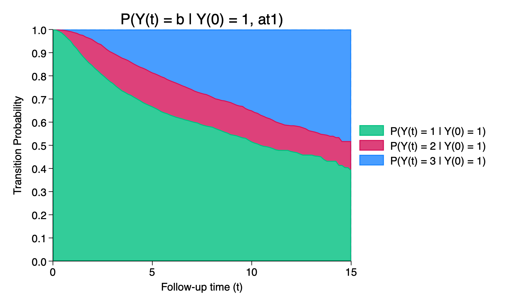
As well as transition probabilities, we can calculate the mean length of time spent in each state, as a function of follow-up time, by adding the los option,
. predictms,      transmatrix(tmat)       ///
>                 models(m1 m2 m3)        ///
>                 probability             ///
>                 los                     ///
>                 at1(age 50)             ///
>                 timevar(tvar)
. list _los_* tvar if inlist(_n,34,67,100)
+------------------------------------------+
| _los_at~1 _los_at~2 _los_at~3 tvar |
|------------------------------------------|
34. | 4.1014629 .51887885 .37965824 5 |
67. | 7.0596484 1.2160731 1.7242785 10 |
100. | 9.374813 1.7923428 3.8328442 15 |
+------------------------------------------+We can get useful contrasts between covariate patterns through use of the at2() option (you can use more at#()s if you wish). Here, we’ll calculate the difference in transition probabilities for a patient aged 60, compared to a patient aged 50 (at1() is the default reference group – you can change that with atreference()),
. predictms,      transmatrix(tmat)       ///
>                 models(m1 m2 m3)        ///
>                 probability             ///
>                 los                     ///
>                 at1(age 50)             ///
>                 at2(age 60)             ///
>                 timevar(tvar)           ///
>                 difference
. list _diff_prob_* tvar if inlist(_n,34,67,100), ab(15)
+------------------------------------------------------------+
| _diff_prob_at~1 _diff_prob_at~2 _diff_prob_at~3 tvar |
|------------------------------------------------------------|
34. | .00441 -.01051 .0061 5 |
67. | -.00306 -.01338 .01644 10 |
100. | -.02906 -.01822 .04728 15 |
+------------------------------------------------------------+Instead of the difference, we could get the ratio,
. predictms,      transmatrix(tmat)       ///
>                 models(m1 m2 m3)        ///
>                 probability             ///
>                 los                     ///
>                 at1(age 50)             ///
>                 at2(age 60)             ///
>                 timevar(tvar)           ///
>                 ratio
The above is brief (we know), and shows the main new additions to functionality. Currently, confidence intervals through the ci option are not supported, but we’re working on this, along with many more developments. Drop us an email to [email protected], for any feedback, feature requests and bug reports.
Latest Resources

Specialist subjects
Clinical Trial Services

Specialist subjects
Methods Development

Specialist subjects